Generative Adversarial Networks: Creating new numbers¶

Imports¶

[1]:

# importing functions and classes from our framework
from dataset import Dataset
from gan import GAN
from layers import Dense
# other imports
import matplotlib.pyplot as plt
import numpy as np
np.random.seed(333)

Theory¶

To be able to understand how a Generative Adversarial Network (GAN) works, let us first start with a similar phenomenon from the real world. Try to imagine that you are an owner of a world-renowned art auction house. Your clients are collecting master pieces of infamous painters, like Pablo Picasso or Vincent Van Gogh. These paintings have very high price tags and thus it has become very lucrative to create cheap replicas. Some of them have even found a way into your auctions. To ensure that your clients receive the original paintings and not some cheap knock-offs, you then ask a friend who has taken some art classes in college to be the judge whether paintings are replicas or the real deal. Fortunately for you, the criminals in your area don’t know too much about art and your friend can sometimes identify forged paintings. A few months pass and your friend doesn’t seem to be able to distinguish between real and fake paintings any more. Furthermore, you now receive a lot of angry letters of your clients which want their money back, since they didn’t want to buy an art forgery. After thinking for a while, you come to the conclusion that the criminals must have gotten better at forging paintings and that your friend’s art classes probably are not sufficient to differentiate between replicas and originals any more. Thus, you hire an art expert to teach your friend the ropes of the art business. Now he is able to detect forgeries again with a decent accuracy, but the criminals are not procrastinating either and are improving their painting skills every day. This power struggle goes back and forth for a long time, until your friend has become an art expert and the criminals have become exceptionally proficient at forging paintings. But what has this story to do with neural networks?

A GAN consists of two neural networks: a generator - the painting forging criminals - and a discriminator - the friend that tries to distinguish whether a painting is real or fake. We will continue by explaining how GANs work by working with the MNIST dataset of handwritten digits. The generator and the discriminator play a minimax game where the generator wants to fool the discriminator and the discriminator wants to detect fakes. This can be expressed in the loss function

Thus we can see that: - the discriminator D tries to label images from the MNIST dataset as real, i.e. learns to assign them a value of 1 - the discriminator D tries to label images that ARE NOT in the MNIST dataset as fake, i.e. learns to assign them a value of 0 - the generator G tries to create images that the discriminator D labels as real, i.e. tries to create images which the discriminator then assigns a value of 1

Demo¶

Now we load a GAN that has been trained on the MNIST dataset. The generator and the discriminator are multi-layer perceptrons.

[2]:

gan = GAN()
gan.load("mnist_gan") # gan is saved in '/models/mnist_gan'
print(gan)

-------------------- GENERATIVE ADVERSARIAL NETWORK (GAN) --------------------

TOTAL PARAMETERS = 2946577

#################
#   GENERATOR   #
#################

 *** 1. Layer: ***
---------------------------------
DENSE 100 -> 256 [LeakyReLU_0.2]
---------------------------------
Total parameters: 25856
---> WEIGHTS: (256, 100)
---> BIASES: (256,)
---------------------------------

 *** 2. Layer: ***
---------------------------------
DENSE 256 -> 512 [LeakyReLU_0.2]
---------------------------------
Total parameters: 131584
---> WEIGHTS: (512, 256)
---> BIASES: (512,)
---------------------------------

 *** 3. Layer: ***
----------------------------------
DENSE 512 -> 1024 [LeakyReLU_0.2]
----------------------------------
Total parameters: 525312
---> WEIGHTS: (1024, 512)
---> BIASES: (1024,)
----------------------------------

 *** 4. Layer: ***
-------------------------
DENSE 1024 -> 784 [Tanh]
-------------------------
Total parameters: 803600
---> WEIGHTS: (784, 1024)
---> BIASES: (784,)
-------------------------

#####################
#   DISCRIMINATOR   #
#####################

 *** 1. Layer: ***
----------------------------------
DENSE 784 -> 1024 [LeakyReLU_0.2]
----------------------------------
Total parameters: 803840
---> WEIGHTS: (1024, 784)
---> BIASES: (1024,)
----------------------------------

 *** 2. Layer: ***
----------------------------------
DENSE 1024 -> 512 [LeakyReLU_0.2]
----------------------------------
Total parameters: 524800
---> WEIGHTS: (512, 1024)
---> BIASES: (512,)
----------------------------------

 *** 3. Layer: ***
---------------------------------
DENSE 512 -> 256 [LeakyReLU_0.2]
---------------------------------
Total parameters: 131328
---> WEIGHTS: (256, 512)
---> BIASES: (256,)
---------------------------------

 *** 4. Layer: ***
-------------------------
DENSE 256 -> 1 [Sigmoid]
-------------------------
Total parameters: 257
---> WEIGHTS: (1, 256)
---> BIASES: (1,)
-------------------------

----------------------------------------------------------------------

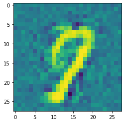
GANs are, as the name suggests, generative models. Hence training it on handwritten digits, we would expect, that it can come up with new numbers by itself. It is difficult to train GANs (see GANs Lessons) and we haven’t implemented regularizers like dropout or batch normalization. Hence we don’t have optimal results. Training a GAN is a highly unstable optimization problem and it is difficult to find the equilibrium between the discriminator and the generator.

It can be seen that the plain output of the generator looks very noisy. This is partially also caused by the activation function in the output layer, which we chose to be the hyperbolic tangent. Thus the output values are between -1 and 1, but usually we would like grayscale values between 0 and 1 (or between 0 and 255).

[4]:

ganImage = gan.generator.feedforward(gan.sample(1))
plt.imshow(ganImage.reshape(28,28))
plt.show()

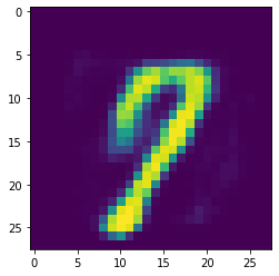
To achieve proper scaling of the image, i.e. values between 0 and 1, we apply ReLU on the entire image.

[5]:

plt.imshow((ganImage * (ganImage > 0.)).reshape(28,28))
plt.show()

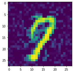
In the previous parts of our project, we have seen that denoising autoencoders are very effective in filtering noise out of images. Hence, we will use a denoising autoencoder after our discriminator to generate noise-free digits.

[7]:

from autoencoder import Autoencoder

ae = Autoencoder()
ae.load("ae_gans") # ae is saved in '/models/ae_gans'
print(ae)

-------------------- MULTI LAYER PERCEPTRON (MLP) --------------------

HIDDEN LAYERS = 0
TOTAL PARAMETERS = 79234

 *** 1. Layer: ***
-----------------------
DENSE 784 -> 50 [ReLU]
-----------------------
Total parameters: 39250
---> WEIGHTS: (50, 784)
---> BIASES: (50,)
-----------------------

 *** 2. Layer: ***
--------------------------
DENSE 50 -> 784 [Sigmoid]
--------------------------
Total parameters: 39984
---> WEIGHTS: (784, 50)
---> BIASES: (784,)
--------------------------

----------------------------------------------------------------------

[6]:

plt.imshow(ae.feedforward(ganImage).reshape(28,28))
plt.show()