Run the code in Google Colab:
FEM code for the Poisson problem in 1D: 
FEM code for the Poisson problem in 2D:
Imports
import numpy as np
from scipy.sparse import dok_matrix
from scipy.sparse.linalg import spsolve
import matplotlib.pyplot as plt
How does the Finite Element Method work?
Deriving the linear equation system for the Poisson equation
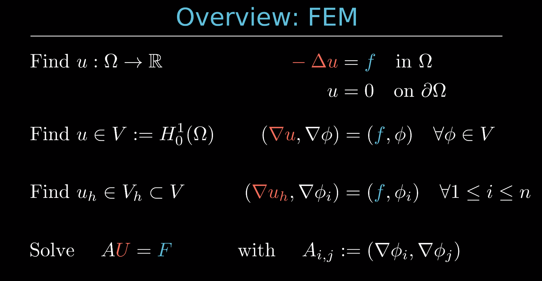
In this notebook, we will show how from the strong form of the Poisson problem
Find $u: \Omega \rightarrow \mathbb{R}$ such that
$$ \qquad u = 0 \quad \text{ on } \partial \Omega $$
you can derive the linear equation system $AU = F$.
We will use the following notation for the $L^2$-inner product:
$$ (f,g) := \int_\Omega f\cdot g\, dx. $$Let the strong form of the Poisson problem be given, which reads
Find $u: \Omega \rightarrow \mathbb{R}$ such that
$$ \qquad u = 0 \quad \text{ on } \partial \Omega $$
In this demonstration we will work with $f = -1$:
# right-hand side
f = -1.0
Then we define the function space $$ V := H^1_0(\Omega ), $$ which means that $V$ contains all functions that are one time (weakly) differentiable and vanish at the boundary ($u = 0 \text{ on } \partial \Omega$).
When we multiply the Poisson equation from the right with a test function $\phi \in V$, we get that
$$ (-\Delta u, \phi) = (f, \phi) \qquad \forall \phi \in V.$$We can then apply integration by parts (Green's theorem) the left side of this equation, which yields
$$ (\nabla u, \nabla \phi) - \int_{\partial \Omega} \partial_n u \phi\, ds = (f, \phi) \qquad \forall \phi \in V.$$Note that since $\phi$ is $0$ at the boundary of the domain $\partial \Omega$, the integral over the boundary is $0$ and thus our weak formulation of the poisson problem reads
Find $u \in V = H^1_0(\Omega)$ such that
We have reduced our PDE to a variational problem, but we are still working with an infinite dimensional function space $V$. Thus in the next step we try to replace $V$ with finite dimensional subspace $V_h$. In the following be will lok at how this could be done in 1D and then we will look at the 2D case.
Discrete weak form in 1D
First we need to discretize our domain $\Omega$ which in 1D is just an open interval. We will deal with the domain $\Omega = (0,1)$ and divide it into subintervals $(x_i, x_i + h)$ where $h$ is a constant, which we call the mesh size. We refer to these subintervals as finite elements or cells.
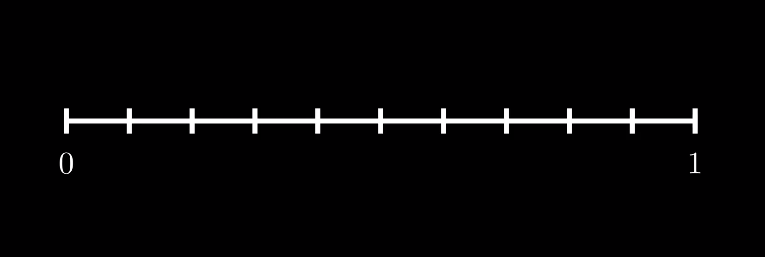
Now, we choose $V_h$ to be the set of functions which are $0$ at the boundary of $\Omega$, i.e. $u(0) = u(1) = 0$, and are linear on each cell $K_i := (x_i, x_i + h)$.
Note: We could also have chosen the functions to be polynomials of $k$.th order on each cell with $k > 1$.
Now a basis of the function space $V_h$ can be derived as follows:
Since the hat functions $\phi_i$ form a basis function of $V_h$, each function in $V_h$ can be expressed as a linear combination of the functions $\phi_i$ and the coefficients in front of these basis functions uniquely identify a function in $V_h$.
For our code, it is not necessary to store all these linear hat functions, but it is sufficient to define what the basis functions on the general element $(0,1)$, the so-called master element, look like:
# basis functions in 1D
hat0 = {"eval": lambda x: x, "nabla": lambda x: 1}
hat1 = {"eval": lambda x: 1 - x, "nabla": lambda x: -1}
hatFunction = [hat0, hat1]
To solve the Poisson problem, we implemented what the function values of these hat functions are and what their derivative is.

Discrete weak form in 2D
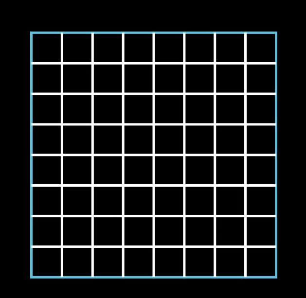
We also try to contruct the finite dimensional function space $V_h \subset V$, in the same way as we did in only one dimension. First we need to discretize our domain $\Omega$. In 2D the domain $\Omega$ can have many different shapes and forms, but for this explanation we will look at the unit square $\Omega = (0,1) \times (0,1)$. The most common ways to discretize a two dimensional domain is to divide it into rectangles or triangles. Here we will divide $\Omega$ into smaller square of width $h$, where $h$ denotes again the mesh size. These smaller square are also called finite elements or cells.
To implement this discretization in code, we construct 3 classes:
- the DoF (degree of freedom), which corresponds to the point where two grid lines intersect,
- the Cell, which have 4 DoFs, one located in each corner (at each vertex) and
- the Grid, which contains all cells and DoFs
class DoF:
    def __init__(self, x, y, ind=-1):
        self.x, self.y = x, y
        self.ind = ind
class Cell:
    def __init__(self, origin, right, up, upRight):
        self.dofs = [origin, right, up, upRight]
The Grid class is a bit more lengthy and we will add some more functions later on. Right now the Grid class only creates the unit square $(0,1) \times (0,1)$ and divides it into cells of width $0.5$. During this discretization of the grid, all DoFs and all Cells are being saved for future computations.
class Grid:
    def __init__(self, xMin=0.0, xMax=1.0, yMin=0.0, yMax=1.0, stepSize=0.5):
        self.xMin, self.xMax = xMin, xMax
        self.yMin, self.yMax = yMin, yMax
        self.h = stepSize
        self.dofs, self.cells = [], []

    def decompose(self):
        # create mesh and transform it into a list of x and y coordinates
        xRange = np.arange(self.xMin, self.xMax, self.h)
        xRange = np.append(xRange, [self.xMax])
        self.xNum = len(xRange)
        yRange = np.arange(self.yMin, self.yMax, self.h)
        yRange = np.append(yRange, [self.yMax])
        self.yNum = len(yRange)
        self.xCoord, self.yCoord = np.meshgrid(xRange, yRange)
        xList, yList = self.xCoord.ravel(), self.yCoord.ravel()

        # create DoFs
        for i, (x, y) in enumerate(zip(xList, yList)):
            self.dofs.append(DoF(x, y, ind=i))

        # create cells
        for i, dof in enumerate(self.dofs):
            if dof.x != self.xMax and dof.y != self.yMax:
                self.cells.append(
                    Cell(
                        dof,
                        self.dofs[i + 1],
                        self.dofs[i + self.xNum],
                        self.dofs[i + self.xNum + 1],
                    )
                )
Now we choose $V_h$ to be the set of functions which are $0$ at the boundary of $\Omega$ and are linear on each cell. For our FEM code it is sufficient to define what the linear hat functions on the master element $(0,1) \times (0,1)$ look like. We can get the two dimensional hat functions by taking the (tensor) product of the one dimensional hat functions on $(0,1)$. This can be seen in the following video:
# basis functions in 2D = tensor product of 1D basis functions
class Phi2D:
    def __init__(self, x0, y0):
        self.xBasis = hatFunction[x0]
        self.yBasis = hatFunction[y0]

    # function evaluation
    def eval(self, x, y):
        return self.xBasis["eval"](x) * self.yBasis["eval"](y)

    # derivative
    def nabla(self, x, y):
        return np.array(
            [
                self.xBasis["nabla"](x) * self.yBasis["eval"](y),
                self.xBasis["eval"](x) * self.yBasis["nabla"](y),
            ]
        )
# linear basis functions in 2D
basisFunction = {0: Phi2D(0, 0), 1: Phi2D(1, 0), 2: Phi2D(0, 1), 3: Phi2D(1, 1)}
From now on, since we have found a finite dimensional subspace $V_h \subset V$, instead of the weak form
Find $u \in V = H^1_0(\Omega)$ such that
we now work with a discrete weak form
Find $u_h \in V_h \subset V(\Omega)$ such that
This is a problem which will be computable for us soon and if we let $h \rightarrow 0$, then $u_h \rightarrow u$. This means that that the solution of our discretized weak form converges to the solution of the weak form.
Converting the discretized weak form into a linear equation system
In the next video, you can see how a linear equation system can be derived from the (discrete) weak form. For this we only use the fact that $\lbrace \phi_i \rbrace_{i = 1}^{n}$ is a basis of $V_h$ and thus each function $u_h \in V_h$ can be expressed as their linear combination of these hat functions, that is
$$ u_h = \sum_{j = 1}^n u_j \phi_j. $$Now we only need to be able determine the entries of the matrix $A$, which means we need to be able to compute
$$A_{ij} = (\nabla \phi_j, \nabla \phi_i) := \int_\Omega \nabla \phi_j \cdot \nabla \phi_i\, dx$$and we also need to determine the entries of the right hand side vector $F$, which means we need to be able to compute
$$F_{i} = (f, \phi_i) := \int_\Omega f \phi_i\, dx.$$If we know $A$ und $F$, then we can just solve the linear system, i.e. $U = A^{-1}F$ and then the solution to the discrete weak form is
$$ u_h = \sum_{j = 1}^n u_j \phi_j = \sum_{j = 1}^n \big(A^{-1}F\big)_j \phi_j. $$Assembling and solving the linear equation system
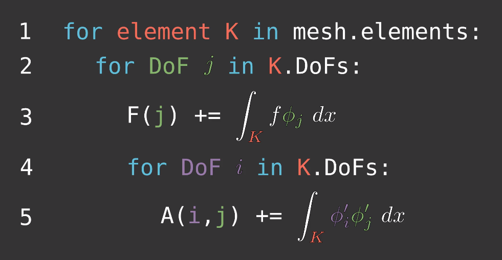
We try to assembly $A$ and $F$ efficiently. The first thing we realize is that we divided the domain $\Omega$ into the cells $K$ and instead of integrating over $\Omega$, we can simply integrate over the individual cells and then sum up the results. In formulae this means that
$$ \int_\Omega \dots\, dx = \sum_{\text{cell } K \in\, \Omega}\, \int_K \dots\, dx.$$At this point we introduce the first real improvement to our algorithm: In all integrals that we are trying to compute the basis functions $\phi_i$ come up. We know that $\phi_i$ is $1$ at the $i$.th DoF and it than goes to $0$ at the neighboring nodes of the $i$.th node. This means that the area on which $\phi_i$ is nonzero is very small, in particular $\phi_i$ is only nonzero on the cells, which contain the $i$.th DoF. Thus we can formulate the following algorithm, in which we only compute those integrals that are possibly nonzero:
There are still two major improvements that can be made to this algorithm: approximating the integrals with numerical quadrature and evaluating all integrals on the master element.
Numerical quadrature
In this video you can see how we can approximate integrals numerically by evaluating the integrand in a finite number of points and weighting these values in a smart way.
If you look at the functions, which need to be integrated to compute $A$ and $F$, you see that these are polynomials of up to second order. It would thus be sensible to use a numerical quadrature scheme, which integrates polynomials up to second order exactly. The Simpson rule is such a scheme with
$$ \int_a^b g(x)\, dx \approx \Big(\dfrac{b-a}{6}\Big)\cdot \Bigg(g(a) + 4g\Big(\dfrac{a+b}{2}\Big) + g(b)\big) \Bigg). $$In our assembly, we will transform all integrals onto the master element in the next step. Thus we will only need to be able to evaluate integrals with $a = 0$ and $b = 1$. Thus the quadrature points and quadrature weights (in our code) are as follows:
# quadrature points and weights
quad = simpson = [(0.0, 1 / 6), (0.5, 4 / 6), (1.0, 1 / 6)]  # simpson rule
Evaluation on master element
In this video, you can learn how in 1D the integrals are being transformed onto the master element $(0,1)$ and how this can applied to the integrals in our assembly together with the numerical quadrature.
If we do the math for the 2D case that we are dealing with, we find that
$$ J = h^2,$$$$ \int_K f(x)\,\phi^K_j(x)\, dx = \int_{M} f(T(\xi))\,\phi^{M}_j(\xi)\, h^2\, d\xi$$and
$$ \int_K \nabla_x\phi^K_i(x)\cdot \nabla_x\phi^K_j(x)\, dx = \int_{M} \nabla_\xi\phi^{M}_i(\xi)\cdot\nabla_\xi\phi^{M}_j(\xi)\, d\xi,$$where $M := (0,1) \times (0,1)$ is the master element and $T$ is the affine transformation from the master element $M$ to a particular cell $K$.
Assembly code
Now that we know how we can compute $A$ and $F$ efficiently, we can program the assembly of the linear equation system by using numerical quadrature and evaluating all integrals on the master element. At the end, we also need to make sure that the solution of our linear equation system satisfies the homogeneous Dirichlet boundary conditions, i.e. $u_h = 0$ on $\partial \Omega$.
def assembleSystem(self):
    # system matrix
    A = dok_matrix((len(self.dofs), len(self.dofs)), dtype=np.float32)
    # system right hand side
    F = np.zeros(len(self.dofs), dtype=np.float32)

    for cell in self.cells:
        for x, y, quadWeight in [ (x, y, wX * wY) for (x, wX) in quad for (y, wY) in quad ]:
            for j, dof_j in enumerate(cell.dofs):
                # assemble rhs
                F[dof_j.ind] += (
                    quadWeight * f * basisFunction[j].eval(x, y) * self.h ** 2
                )
                for i, dof_i in enumerate(cell.dofs):
                    # assemble matrix
                    A[dof_i.ind, dof_j.ind] += quadWeight * basisFunction[i].nabla(x, y).dot(
                        basisFunction[j].nabla(x, y)
                    )

    # apply homogeneous Dirichlet boundary conditions
    for dof in self.dofs:
        if dof.x in [self.xMin, self.xMax] or dof.y in [self.yMin, self.yMax]:
            _, nonZeroColumns = A[dof.ind, :].nonzero()
            for j in nonZeroColumns:
                A[dof.ind, j] = 0.0
            A[dof.ind, dof.ind] = 1.0
            F[dof.ind] = 0.0

    return A.tocsr(), F

Grid.assembleSystem = assembleSystem
Code for plotting the solution
Finaylly we also might be interested in what the solution looks like. For this we created the following function, which outputs the contour plot of our FEM solution $u_h$.
def plotSolution(self, solution):
    fig = plt.figure(figsize=(10,10))
    # 2D contour plot
    plt.contourf(
        self.xCoord,
        self.yCoord,
        solution.reshape(self.yNum, self.xNum),
        20,
        cmap="viridis",
    )
    plt.colorbar()
    plt.show()

Grid.plotSolution = plotSolution
Solve linear equation system
Now that we talked about the derivation of the linear equation system and how this can be implemented in code, we can finally run our simulation and solve the Poisson problem numerically.
grid = Grid(stepSize = 0.05)
grid.decompose()
A, F = grid.assembleSystem()
solution = spsolve(A, F)  # U = A^{-1}F
grid.plotSolution(solution)
